Approximate when you are going to die

Question

A mortality table or life table is an actuarial tool that gives the probability that a person aged \$A\$ years will die in the next year, and is used to help calculate the premiums for life insurance, among other things. One of the first people to compile a life table was Edmond Halley, of cometary fame. These probabilities also allow you to estimate the life expectancy for a given age, which is the goal of this challenge.

Input

• An integer from 0 to 119, inclusive.
• An indicator for Sex M/F.

Output

• An approximation for the life expectancy for that Age/Sex according to the Social Security Administration's 2016 Mortality Table, aka the Actuarial Life table, the relevant part of which can be found below.

Age     M           F
0       75.97       80.96
1       75.45       80.39
2       74.48       79.42
3       73.50       78.43
4       72.52       77.45
5       71.53       76.46
6       70.54       75.47
7       69.55       74.47
8       68.56       73.48
9       67.57       72.49
10      66.57       71.50
11      65.58       70.50
12      64.59       69.51
13      63.60       68.52
14      62.61       67.53
15      61.63       66.54
16      60.66       65.55
17      59.70       64.57
18      58.74       63.59
19      57.79       62.61
20      56.85       61.63
21      55.91       60.66
22      54.98       59.69
23      54.06       58.72
24      53.14       57.75
25      52.22       56.78
26      51.31       55.82
27      50.39       54.85
28      49.48       53.89
29      48.56       52.93
30      47.65       51.97
31      46.74       51.01
32      45.83       50.06
33      44.92       49.10
34      44.01       48.15
35      43.10       47.20
36      42.19       46.25
37      41.28       45.30
38      40.37       44.36
39      39.47       43.41
40      38.56       42.47
41      37.65       41.53
42      36.75       40.59
43      35.85       39.66
44      34.95       38.73
45      34.06       37.80
46      33.17       36.88
47      32.28       35.96
48      31.41       35.04
49      30.54       34.13
50      29.67       33.23
51      28.82       32.33
52      27.98       31.44
53      27.14       30.55
54      26.32       29.68
55      25.50       28.81
56      24.70       27.94
57      23.90       27.09
58      23.12       26.24
59      22.34       25.39
60      21.58       24.56
61      20.83       23.72
62      20.08       22.90
63      19.35       22.07
64      18.62       21.26
65      17.89       20.45
66      17.18       19.65
67      16.47       18.86
68      15.77       18.07
69      15.07       17.30
70      14.39       16.54
71      13.71       15.79
72      13.05       15.05
73      12.40       14.32
74      11.76       13.61
75      11.14       12.92
76      10.53       12.23
77      9.94        11.57
78      9.37        10.92
79      8.82        10.29
80      8.28        9.68
81      7.76        9.09
82      7.26        8.52
83      6.79        7.98
84      6.33        7.45
85      5.89        6.95
86      5.48        6.47
87      5.08        6.01
88      4.71        5.57
89      4.37        5.16
90      4.05        4.78
91      3.75        4.43
92      3.48        4.11
93      3.23        3.81
94      3.01        3.55
95      2.81        3.31
96      2.64        3.09
97      2.49        2.90
98      2.36        2.73
99      2.24        2.58
100     2.12        2.42
101     2.01        2.28
102     1.90        2.14
103     1.80        2.01
104     1.70        1.88
105     1.60        1.76
106     1.51        1.65
107     1.42        1.54
108     1.34        1.44
109     1.26        1.34
110     1.18        1.24
111     1.10        1.15
112     1.03        1.06
113     0.96        0.98
114     0.90        0.91
115     0.84        0.84
116     0.78        0.78
117     0.72        0.72
118     0.66        0.66
119     0.61        0.61

For convenience, here they are in wide form (ages 0-119 in order):

M: [75.97, 75.45, 74.48, 73.5, 72.52, 71.53, 70.54, 69.55, 68.56, 67.57, 66.57, 65.58, 64.59, 63.6, 62.61, 61.63, 60.66, 59.7, 58.74, 57.79, 56.85, 55.91, 54.98, 54.06, 53.14, 52.22, 51.31, 50.39, 49.48, 48.56, 47.65, 46.74, 45.83, 44.92, 44.01, 43.1, 42.19, 41.28, 40.37, 39.47, 38.56, 37.65, 36.75, 35.85, 34.95, 34.06, 33.17, 32.28, 31.41, 30.54, 29.67, 28.82, 27.98, 27.14, 26.32, 25.5, 24.7, 23.9, 23.12, 22.34, 21.58, 20.83, 20.08, 19.35, 18.62, 17.89, 17.18, 16.47, 15.77, 15.07, 14.39, 13.71, 13.05, 12.4, 11.76, 11.14, 10.53, 9.94, 9.37, 8.82, 8.28, 7.76, 7.26, 6.79, 6.33, 5.89, 5.48, 5.08, 4.71, 4.37, 4.05, 3.75, 3.48, 3.23, 3.01, 2.81, 2.64, 2.49, 2.36, 2.24, 2.12, 2.01, 1.9, 1.8, 1.7, 1.6, 1.51, 1.42, 1.34, 1.26, 1.18, 1.1, 1.03, 0.96, 0.9, 0.84, 0.78, 0.72, 0.66, 0.61]
F: [80.96, 80.39, 79.42, 78.43, 77.45, 76.46, 75.47, 74.47, 73.48, 72.49, 71.5, 70.5, 69.51, 68.52, 67.53, 66.54, 65.55, 64.57, 63.59, 62.61, 61.63, 60.66, 59.69, 58.72, 57.75, 56.78, 55.82, 54.85, 53.89, 52.93, 51.97, 51.01, 50.06, 49.1, 48.15, 47.2, 46.25, 45.3, 44.36, 43.41, 42.47, 41.53, 40.59, 39.66, 38.73, 37.8, 36.88, 35.96, 35.04, 34.13, 33.23, 32.33, 31.44, 30.55, 29.68, 28.81, 27.94, 27.09, 26.24, 25.39, 24.56, 23.72, 22.9, 22.07, 21.26, 20.45, 19.65, 18.86, 18.07, 17.3, 16.54, 15.79, 15.05, 14.32, 13.61, 12.92, 12.23, 11.57, 10.92, 10.29, 9.68, 9.09, 8.52, 7.98, 7.45, 6.95, 6.47, 6.01, 5.57, 5.16, 4.78, 4.43, 4.11, 3.81, 3.55, 3.31, 3.09, 2.9, 2.73, 2.58, 2.42, 2.28, 2.14, 2.01, 1.88, 1.76, 1.65, 1.54, 1.44, 1.34, 1.24, 1.15, 1.06, 0.98, 0.91, 0.84, 0.78, 0.72, 0.66, 0.61]

Scoring Rules

For this challenge, the submission with the lowest score wins. Your score will be equal to \$(1+L)\times(1 + M)\$, where \$L\$ is the length of your code in bytes and \$M\$ is the mean-squared error of your estimates, rounded to two decimal places. This is a scoring program for \$M\$.

Other rules

• Standard loopholes are forbidden.
• Input is pretty flexible. You can specify any two distinct values for M/F: 'M'/'F',0/1. If you really wanted, you could even take a single integer, with the sign representing M/F, but note that 0 is an input for both. Or the real and imaginary parts of a complex number.
  • You don't have to take any input if you don't want, which should allow you to post answers that just always return 4 or whatever.
• In case there was any confusion, the output cannot be random.
• Please include a means of verifying your score.
• Builtins that have this exact mortality table are not banned, but do please implement your own solution as well.
• Explanations are encouraged.

Additional Bonuses:

Since R is the language of the month for September 2020, I will be awarding a 500 rep bounty to the R answer with the best score at the end of the month.

Answer 1

JavaScript (ES6), Score:  59.51  59.10

L = 52 bytes, M ≈ 0.1150638

Expects (n)(m), where m is 1 for Male or 0 for Female.

n=>m=>81-5*m-(.9+m/51+(70-27*m-(.92-m/7)*n)/2e4*n)*n

Try it online!

or Get the raw data in the format expected by the scoring program.

Method

This is based on two cubic regressions, with a trade-off between code size and accuracy.

For women, this computes:

$$f_0(x)=81-\frac{9}{10}x-\frac{7}{2000}x^2+\frac{23}{500000}x^3$$

And for men:

$$f_1(x)=76-\frac{469}{510}x-\frac{43}{20000}x^2+\frac{17}{437500}x^3$$

How accurate is it?

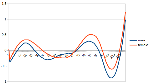
Below is a graph of the errors produced by the function according to the age and the sex.

Answer 2

R, score=67.47 47.92

30 bytes, MSE = 0.54587

-1 byte (and -1.47 in score) thanks to Dominic van Essen.

pnorm(scan(),31,41,F)*scan()-2

Try it online!

The input format is: age as an integer, then a newline, then sex, then a newline. Sex is encoded as 98 for men and 106 for women.

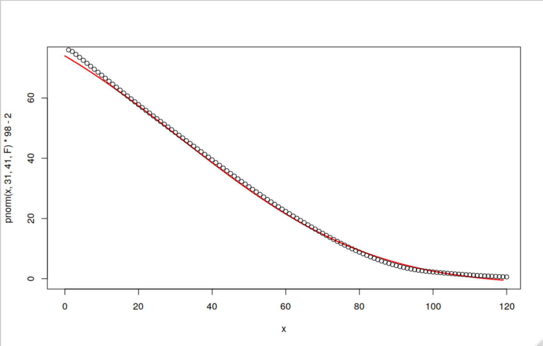
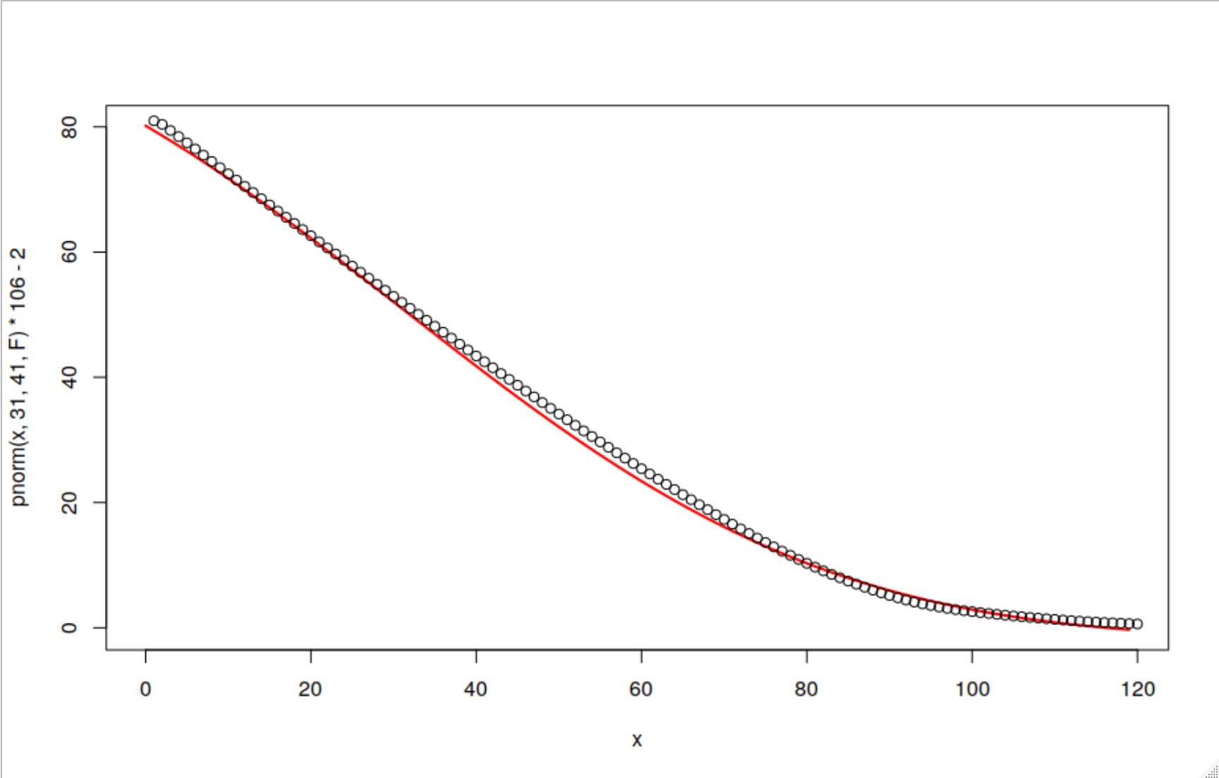
Approximates the actuarial tables by the survival function of a normal distribution (the survival function is 1 - the cumulative distributions function). I tried a few families of distribution, and the normal minimized the MSE.

Let \$\phi(x;\mu,\sigma)\$ be the density of a \$\mathcal N(\mu,\sigma^2)\$ distribution. The approximation used is

\$f(x)=a+m\int_x^\infty\phi(t;\mu,\sigma)\,dt\$

I tried using different parameter values for men and women, but the best score is obtained by using the same values of \$a\$, \$\mu\$ and \$\sigma\$, and picking only different values for \$m\$. Since \$m=98\$ for men and \$m=106\$ for women are the optimal values, I use those to encode the sex directly.

(Actually, the optimal values would be \$m=98.25528\$ for men and \$m=106.34315\$ for women, but using such values to define the sexes really feels like cheating. It would lead to a score of 47.49, a slight improvement.)

Plot of the approximation for men:

Plot of the approximation for women:

Answer 3

Wolfram Language (Mathematica), Score 151.8,

32 bytes, 3.6 MSE

#-Cos[x(Pi-.02)/238]~Sum~{x,#2}&

Try it online!

I noticed that the differences of the values were similar to Cos(x) [0,pi/2]
So, accumulated Cos(x) works pretty good on men...

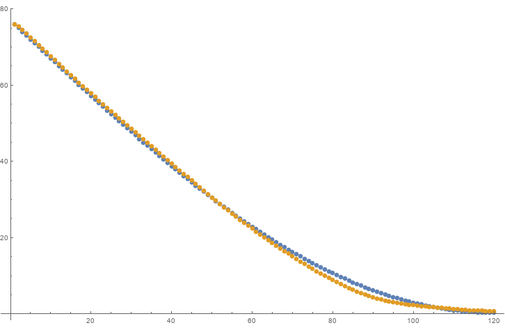
MALE
MSE 0,90

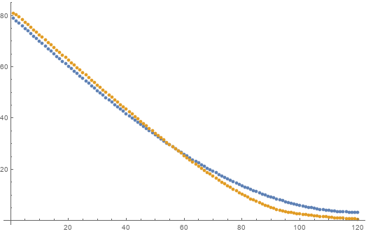
FEMALE
MSE 6,29
(I guess Cos(x) understands men better...)

Special thanks to @att for golfing my code down to 33 bytes

Answer 4

Ruby, score ^{56.12...43.94} 43.92

\$L=35\$, \$M\approx0.220060\$

->x,f{f.*1.87e6-(21676+(66-x)*x)*x}

Try it online!

Input is an age \$x\$ and a float \$f\$, which is 4.027e-5 for male and 4.362e-5 for female. (See below for an alternative version that takes \$f\$ as an integer instead.) The approach is to fit a cubic polynomial to the life expectancy averaged across both sexes, then scale this polynomial by a sex factor to recover sex-specific approximations. The polynomial selected for the average life expectancy is $$ \frac{x^3-66x^2-21676x+1870000}{23840} $$ and the sex factor is $$ \begin{cases}0.96,\;\text{male}\\1.04,\;\text{female}.\end{cases} $$ In other words, the life expectancy of a male is approximately \$0.96\$ times that of an average human (male or female). Similarly, the life expectancy of a female is approximately \$1.04\$ times that of an average human.

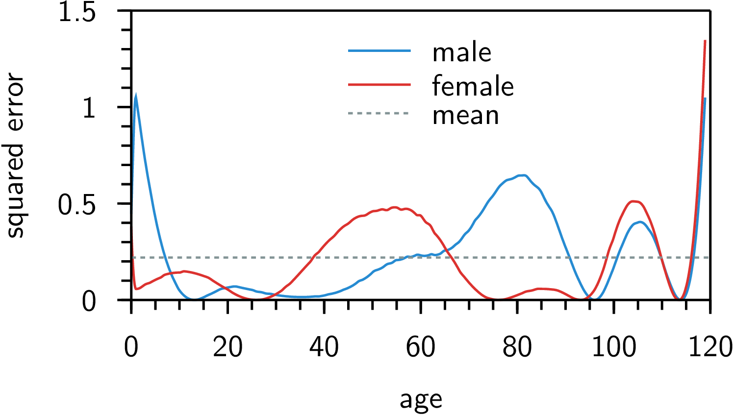
The plot below shows the squared error as a function of age for each sex. The dashed grey line represents the mean squared error for both sexes.

One point of interest in the code is the explicit call to the * method of the float f. Everything to the right of f.* is interpreted as the method argument, so the polynomial doesn't need to be enclosed in parentheses.

---

Ruby, score 50.06

\$L=40\$, \$M\approx0.220981\$

->x,f{f/9e3*(56541-(656+(2-x/33r)*x)*x)}

Try it online!

Despite being within the rules, taking \$f\$ as a float (as above) feels more than a little 'cheaty'. This version uses the same general approach, but here \$f\$ is an integer: \$12\$ for male and \$13\$ for female. The polynomial used for the average life expectancy is $$ \frac{x^3/33-2x^2-656x+56541}{720}. $$

Answer 5

J, score ^53.76 52.78

L = 46, M = 0.122983

Takes M/F as 1/0 on the right side and age on the left side. A simple third degree polynomial approximation. The J polynomials read from left to right, so 81 - 0.9x - 347e-5x² + 455e-7x³ for the 1 case. The 0 case just modifies the numbers a little bit to 76 - 0.92x - 207e-5x² + 385e-7x³. p. evaluates the polynomial at x, in this case the age.

p.~81 _0.9 _347e_5 455e_7-5 0.02 _14e_4 7e_6&*

Try it online!

Answer 6

Python 3, score 94.40, 58 bytes, 0.60 MSE

Just simple linear approximations. True for female and False for male.

lambda a,g:[75+5*g-(.89+g/30)*a,12-a/11][a>81]+(70<a<90)*2

Try it online!

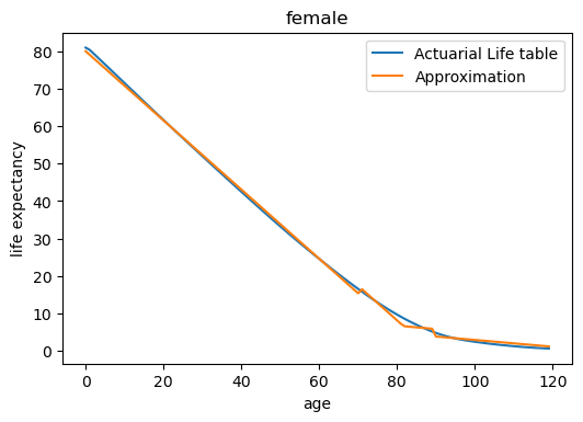
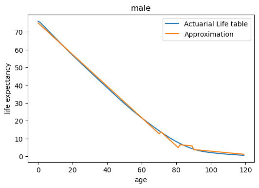
Visual representation of the approximation:

Answer 7

R, score 46.00036

Pushing the limits of 'any two distinct values' as input more than somewhat...

45 bytes, mean-squared-error 7.9e-6

function(a,s)s%/%gmp::as.bigz(1e4)^a%%1e4/100

Try it online!

Input is an integer a as age, and one of two 'big integer' values s to specify M/F sex.
Output is a 'big rational' number.

As (presumably) encouraged by the generously-flexible input rules, the sex-specifying values are integral for the calculation (although in this case probably more so than intended...).
Each of M,F big integers are constructed as the 1...120th power of 1e4 multiplied by 100x the life expectancy at each age: essentially, a base-10000-encoding. The life_expectancy function simply decodes the ath base-10000 digit and divides by 100.

Even though the function uses the arbitrary-precision gmp library for calculations, a small number of the decoded values still contain inaccuracies at the 2nd decimal place, for reasons that I don't understand.
Nevertheless, the mean-squared-error is (as expected) sufficiently close to zero that this doesn't matter, since we need to add 1 to it anyway to get the score.

Answer 8

R, score 75.74445

61 bytes, mean-squared-error 0.222

function(a,s)s*predict(loess(c(82,58,35,14,3,1)~c(0:5*24)),a)

Try it online!

Uses loess smoothing to interpolate between hard-coded data points.

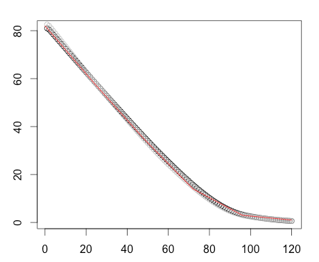
The M and F curves are remarkably similar to each other after scaling (by 0.92x) - see the black & grey points on the graph - so the hard-coded points are taken from the mean of the two (scaled) curves, and then rounded to nice, short values. The red line on the graph shows the interpolated values.

Unfortunately (for me), the scoring system of adding 1 to the mean-square-error strongly rewards reasonably-close fits, but doesn't give very much more reward for a very-close-fit, so the extra code-length here means that the overall score is still worse than Robin Ryder's looser fit to a normal distribution.

Answer 9

Wolfram Language (Mathematica), score 34.16

27 bytes, mean square error 0.21676 (rounded to 0.22)

#3(#2-#+Sqrt[(#2-#)^2+#4])&

Try it online!

An unnamed function (which we will call f for the purposes of discussion) which takes two arguments (in this order), the age (an integer from 0 to 119) and the indicators for female or male in this form:

• indicator for "female": Sequence[83.506,0.4794,222.8]
• indicator for "male": Sequence[80.596,0.4636,248.5]

In Mathematica, f[a,Sequence[b,c,d]] is the same as f[a,b,c,d]; so Sequence[b,c,d] is almost exactly an ordered triple, except it's better for plugging into functions.

The above code implements the mathematical function

\$ f(a,b,c,d) = c\big( b-a + \sqrt{(b-a)^2+d} \big), \$

where \$a\$ is the age and \$b,c,d\$ are numerical parameters used to optimize the fit with the data.

This specific form was motivated by my perception that the graphs of the data for each sex looked like a hyperbola with a slant asymptote to the left and a horizontal asymptote to the right, which can be brought into the above parametric form (here \$(b,0)\$ are the coordinates of the center of the hyperbola, \$2c\$ is the slope of the slant asymptote, and \$d\$ controls how far from the center the hyperbola bends). An evolutionary algorithm was then used to fine-tune the parameters for each sex separately; experiments suggest that there is a single local minimum for each set of data, as all attempts converged to very similar values for \$b,c,d\$.

(Technically, the entire function could have been used as the sex indicator, leading to the 4-byte solution #2@# with score 6.1. But many of the submissions could have done similar things.)