CJam, 28 27 bytes
PP+mr_mc\ms]1.mrmqf*"(,)".\
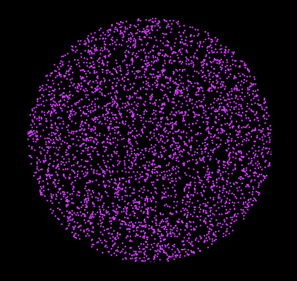
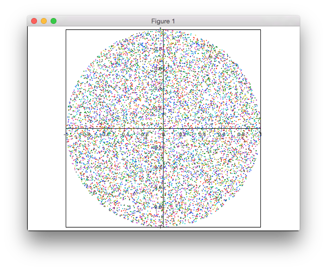
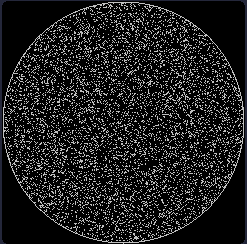
This solution is not rejection-based. I'm generating the points in polar coordinates, but with a non-uniform distribution of the radii to achieve a uniform density of the points.
Test it here.
Explanation
PP+     e# Push 2π.
mr_     e# Get a random float between 0 and 2π, make a copy.
mc\     e# Take the cosine of one copy and swap with the other.
ms]     e# Take the sine of the other copy and wrap them in an array.
        e# This gives us a uniform point on the unit circle.
1.mr    e# Get a random float between 0 and 1.
mq      e# Take the square root. This is the random radius.
f*      e# Multiply x and y by this radius.
"(,)".\ e# Put the resulting numbers in the required format.
Why does it work? Consider a narrow annulus of radius r and (small) width dr. The area is approximately 2π*r*dr (if the annulus is narrow, the inner and outer circumference are almost identical, and the curvature can be ignored, such that the area can be treated as that of a rectangle with side lengths of the circumference and the width of the annulus). So the area increases linearly with the radius. This means that we also want a linear distribution of the random radii, in order to achieve a constant density (at twice the radius, there is twice as much area to fill, so we want twice as many points there).
How do we generate a linear random distribution from 0 to 1? Let's look at the discrete case first. Say, we have a desired distribution of 4 values, like {0.1, 0.4, 0.2, 0.3} (i.e. we want 1 to be 4 times as common as 0, and twice as common as 2; we want 3 three times as common as 0):
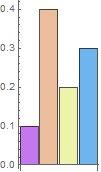
How can pick one of the four values with the desired distribution? We can stack them up, pick a uniformly random value between 0 and 1 on the y-axis and pick the segment at that point:
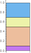
There's a different way to visualise this picking though. We could instead replace each value of the distribution with the accumulation of the values up to that point:
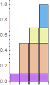
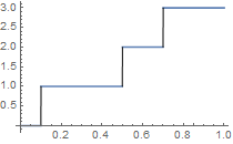
And now we treat the top line of this chart as a function f(x) = y and invert it to get a function g(y) = f-1(y) = x, which we can apply to a uniformly random value in y ∈ [0,1]:
Cool, so how can make use of this to generate a linear distribution of radii? This is the distribution we want:
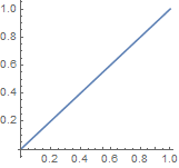
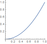
The first step is to accumulate the values of the distribution. But the distribution is continuous, so instead of summing over all previous values, we take an integral from 0 to r. We can easily solve that analytically: ∫0r r dr = 1/2 r2. However, we want this to be normalised, i.e. to multiply it by a constant such that this gives 1 for the maximum value of r, so what we really want is r2:
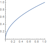
And finally, we invert this to get a function we can apply to a uniform value in [0,1], which we can again do analytically: it's just r = √y, where y is the random value:
This is a fairly useful technique that can often be used to generate simple distributions exactly (it works for any distribution, but for complicated ones the last two steps may have to be solved numerically). However, I wouldn't use it in this particular case in production code, because the square root, sine and cosine are prohibitively expensive: using a rejection-based algorithm is on average much faster, because it only needs addition and multiplication.


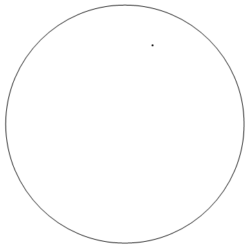

0.3503082505747327+0.13499221288682994j. \$\endgroup\$